User Manual

API Documentation is in working progress.

A Quickstart to UNAMalla 6β v0.3

1. Extract the source code

2. Run Julia and start Pluto

julia> using Pluto; run();

3. Approximate the region boundary using our Pluto Notebook for EditBoundary.

• Search within Pluto the file unamalla6_beta_v0.3\EditBoundary_Notebook.jl and press ENTER.

• Follow the instructions in the notebook.

• Return to the Pluto Menu afterwards.

4. Mesh the region using our Pluto Notebook for UNAMalla.

• Search within Pluto the file unamalla6_beta_v0.3\UNAMalla_Notebook.jl and press ENTER.

• Follow the instructions in the notebook.

A Quickstart to UNAMalla 6β v0.1-0.2

The main routines of the system are organized by sections in a Jupyter Notebook. Run the cells to execute these routines. Mesh generation is carried out interactively through file dialogs, menus, text input, and mouse clicks on plots.

1. Extract the source code and the test regions.

2. Run Julia and start a Jupyter notebook via IJulia.

julia> using IJulia; notebook();

3. Lauch our notebook. Search the UNAMalla6_beta directory inside Jupyter, and then click on the file MENU.ipynb inside this directory.

4. Load the required packages and data structures.

push!(LOAD_PATH,pwd()); include("LOAD_UNAMALLA.jl");

5. Create your own region (Optional)

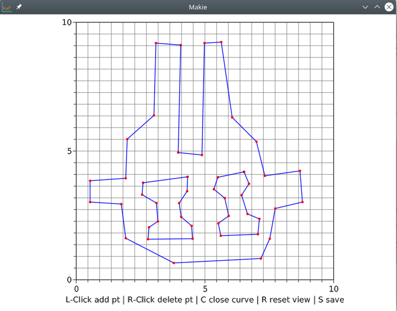
contour_creator_menu()

Press ENTER to use the default option. A new window will be displayed to create your polygonal region by pressing keys and clicking the mouse. Once you draw the exterior boundary, holes can be added in the same fashion.

5. Edit Boundary: Module to approximate polygonal contours

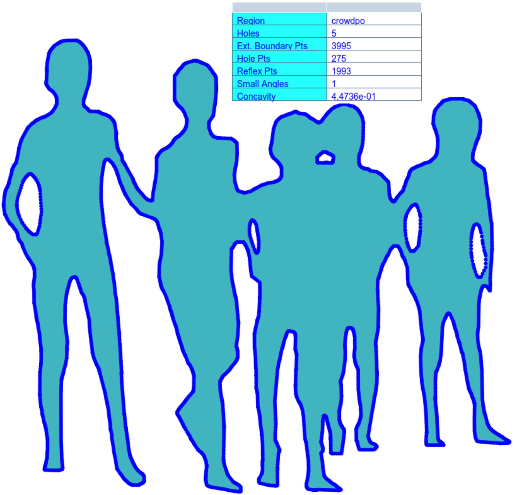
edit_boundary()

A pop-up file dialog appers to select a region. Then, a menu, a plot, and a table will be displayed. The plot and the table change when the boundary is edited or approximated.

1. Click on the Boundary Approx button.
2. Click on the Automatic Approx button.
3. Click on the Save button to save the last approximation.

First Menu of Edit Boundary Region Plot and Info Table Second Menu of Edit Boundary Plot of Boundary Approximation and Comparison Table

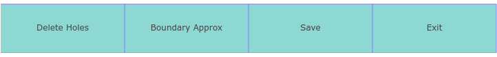
Other avaliable options:

• delete holes. Use this option for regions with several holes.

• Smoothing. Apply further smoothing on a curve chosen by mouse click.

• Edit by clicks Add, delete or move points by pressing keys or mouse clicks.

• Reset sets the last approximation to the original boundary.

• Add Points

6. Interactive decomposition of the region into blocks

interactive_decomposition(MeshDict.Dreg);

Split a region into two blocks by cuts.

1. Click on the show/cut region button.
2. Click on a block of the region decomposition.
3. Click on two boundary points of the block to make a cut.

The plot will be updated with the chosen block or the new region decomposition. Repeat these steps until you get approximately convex blocks without holes nor large peaks.

Region Decomposition Menu Region Decomposition Plot A block with red colored cuts

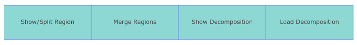
• Four points are needed to split a region with a hole. The points must be chosen so that the hole is connected to the exterior boundary by two cuts.

• If you need to undo a cut, click on the Merge Regions button, and then click on two blocks of the region decomposition plot

• Linux users can use DUDE2D for automatic region decomposition. It is recommend to modify the region decomposition using the interactive mode.

7. Interactive generation of compatible meshes

meshgen(MeshDict);

1. Press ENTER to let the system choose four boundary points (corners) in each block.
2. Click on the Get mesh sizes button to get compatible mesh sizes.
3. Introduce the mesh density factor to generate structured meshes.

A block with its four corners marked by green crosses A structured mesh on the previous block Block structured mesh on the whole region

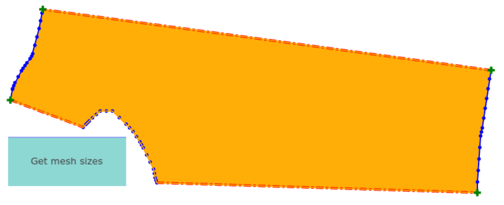
The corners can be changed by mouse clicks before and after the meshes are generated:

1. Click on a block/mesh of the region decomposition/block mesh
2. Click on the block/structured mesh, and then click on four boundary points.
3. Click again on the Get mesh sizes button to update the meshes after changing the corners.

8. Join the structured meshes into a single block mesh

mesh_merging(MeshDict);

Generate a merging order for the meshes and let the system test it. There are three options:

• Automatic mode. The system generates a merging order.

• Interative mode. Generate a merging order by mouse clicks on consecutive blocks.

• Load an order. You already have generated an admissible merging order.

The block mesh is displayed if the test runs without errors.

Note: Use the interactive mode for regions with holes.

Mesh Merging Menu Interactive Mode: Meshes are drawn on the blocks by mouse cliks

9. Mesh Smoothing (the last step)

smoothing_menu(MeshDict);

Just click on the Start button for automatic smoothing of each structured mesh (local smoothing), then the block mesh is smoothed on the whole region (global smoothing).

Mesh Smoothing Menu

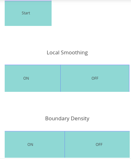
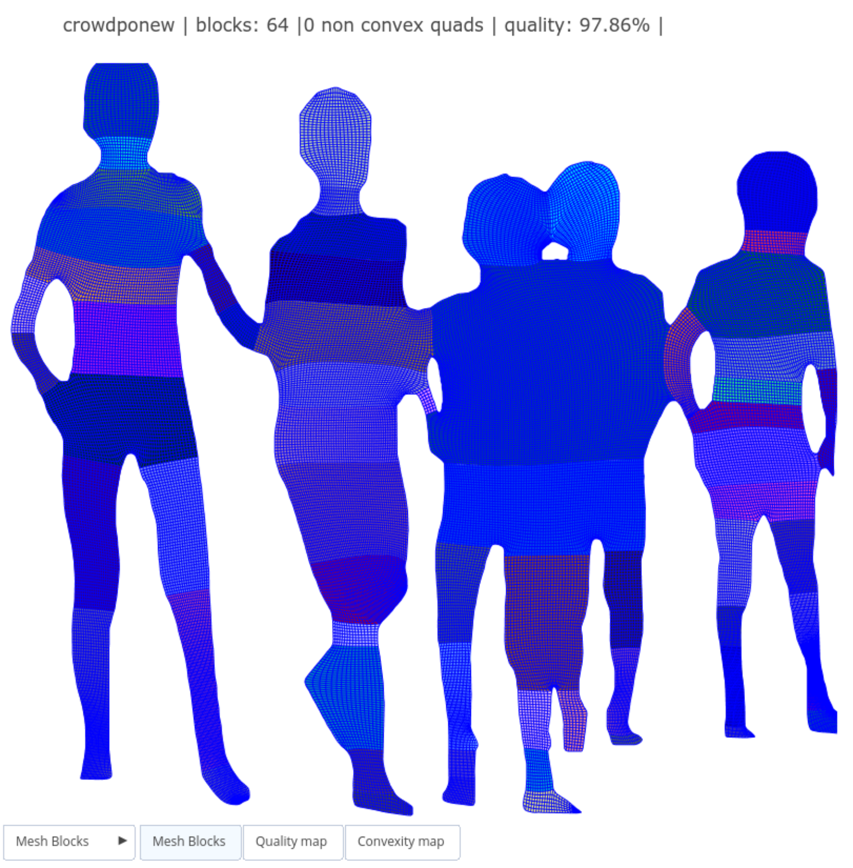
The plot is updated with the smoothed mesh. Click on the attached menu to change the mesh view.

Smoothed block structured mesh on the whole region

Automatic Region Decomposition

Use DUDE2D: A C++ program for automatic region decompostion of polygons. Before you continue, go to the step 6 of the Installation Instructions.

1. Add a new cell in the jupyter notebook with the following instruction:

MeshDict.Dreg = dude2d(get_region());

2. Run this new cell and press ENTER to use the default option or introduce a value for the parameter.

DUDE2D splits irregular shapes into approximately convex blocks using a concavity parameter $\tau\in(0,1)$. This method can be used as auxiliary tool. However, some blocks may lead to poor quality meshes. Merge and split blocks in order to improve the mesh quality.

Input and Output Files

The UNAMalla6_beta_v0.1 directory includes a subdirectory named tests. The system looks for region and mesh files inside this directory. The blocks, meshes, info, and figures of a region are automatically saved in a subdirectory of tests of the same name.

Supported formats for regions:

• XYZ files in which the first polygon is the exterior boundary and the other polygons are holes.

• GEO files generated by our system can be loaded in the mesh generator Gmsh, but not conversely.

Supported format for meshes:

• Structured meshes of each block and the block meshes are saved in MSH format compatible with Gmsh. Only the MSH files generated by UNAMalla 6β can be loaded in our system.

Pipeline for Block Structured Mesh Generation

Mesh generation is carried out in consecutive phases.

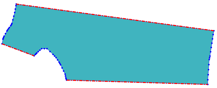
1. Preprocessing: Boundary Approximation

Some regions may have several holes and redundant points, or even noise. Computational problems on these regions are computationally expensive. So the region boundary is approximated by polygonal curves which preserve the shape of the region and essential features with fewer points.

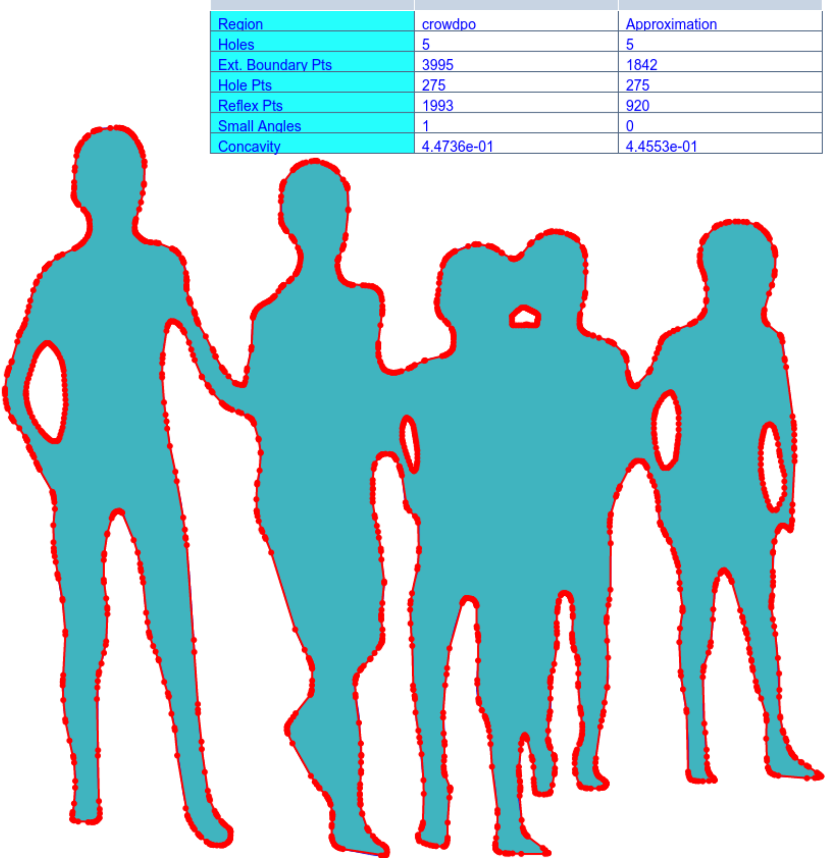
We approximate the region boundary as follows:

• Hole removal: Tiny and irrelevant holes are removed.

• Smoothing: Noise in the boundary is reduced and misaligned points are fixed.

• Point Elimination: Geometric tests are carried out to delete redundant points.

2. Region Decomposition

Polygonal regions with irregular shapes are recursively decomposed into approximately convex regions without holes nor large peaks. In each step the region is split into two polygonal regions by cuts. The key step is the cut choice:

• One cut either to remove peaks or to connect a boundary point far from the convex hull boundary.

• Two cuts to connect a hole with the exterior boundary.

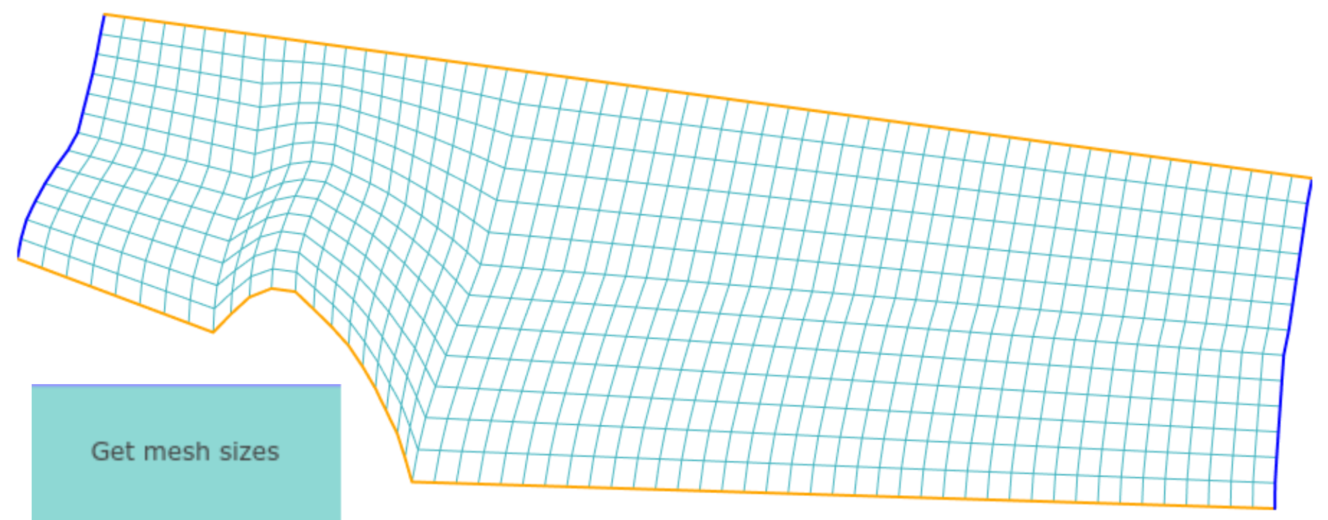
3. Compatible Mesh Sizes

Once we get a suitable region decomposition, we generate matching structured meshes on the blocks. First, we choose the corners of each block and then the mesh density factor. Afterwards we get compatible mesh sizes by solving an interior program. The initial matching meshes are generated by transfinite interpolation (TFI).

4. Mesh Merging

The structured meshes are recursively merged into a global mesh without repeated points. In each step a block structured mesh $G$ is merged with a structured mesh $G_i$ in each step.

The merging order is given by a spanning tree associated to the graph of the region decomposition.

5. Mesh Smoothing

Block structured meshes constructed by TFI may have poor mesh quality. So these meshes are smoothed by a discrete variational approach:

The functional is chosen so that it generates and preserves convex quads as well as it generates quads with approximate right angles and the same approximate area.

Mesh smoothing is carried out in two stages:

• Local Smoothing. In each block the structured mesh is smoothed.

• Global Smoothing. Pairs of meshes sharing a cut are consecutively smoothed.

Suggestions for Block Structured Meshing

1. Delete small holes and smooth the region with fewer points.

2. Undo self-intersections and enlarge bottle necks.

3. Add enough points on large segments to make suitable cuts.

4. Whenever possible, avoid the following features in the region decomposition:

   • huge and tiny blocks (you get huge meshes on huge blocks by mesh size compatibility)

   • blocks with small angles in the cuts (mesh quality is poor on these blocks)

   • hole points which incide with two or more cuts (the mesh merging can be tricky around these holes)

5. Choose corners so that opposite curves of a block boundary have approximately the same length.

6. Generate moderate mesh sizes, $150\times 150$ or below is recommended since the mesh smoothing is memory and time consuming for huge meshes and even the notebook may crash. Change corners or even go back to modify the region decomposition in order to get smaller mesh sizes.

7. Mesh merging may fail in some regions with holes. However it can be fixed by a proper change either from the merging order or from the region decomposition.

8. Turn off the local smoothing only if you have generated smoothed meshes for each block.

Steps to Lauch UNAMalla 6β in your Live USB

The following steps require our ISO image flashed to your USB drive. See

1. Restart your computer with the USB drive attached while pressing a special key (e.g. F2, F5 or F12) to access your Boot menu.

2. In your Boot menu change the order sequence to put first your USB drive. Save changes and exit. The Linux Operating System should automatically start a session afterwards.

3. Inside the session, click on the Jupyter icon located in the sidebar panel. This will lauch Jupyter in a web browser.

4. Navigate to the directory Documents/unamalla6beta and click on the file MENU.ipynb. This will lauch our notebook for UNAMalla 6β.

Now, follow the Quickstart in order to use UNAMalla 6β. Before you exit, copy the content of the directory tests inside the directory Live-usb-storage to save your meshes and figures.

Note: Don't use the routine contour_creator_menu() or the button edit by clicks in the Live USB version since the plots may freeze the system.